Reinforcement Learning Implementation Tips and Tricks

Deep Reinforcement Learning (DRL) implementations often use a variety of tricks that are important for performance and stability, but it can be difficult for newcomers to find these tricks or explanations for how they work. This blog post provides an overview of the tips and tricks we use regularly in our DRL implementations. Our aim is to provide some insight into some of the techniques you could use to improve performance, stability, and compute time of your RL algorithms. We illustrate how to implement the techniques with code snippets using Python and PyTorch.
The tricks in this post are divided into three sections:
- Input formatting - tricks to process inputs before feeding into a neural network
- Optimisation stability - tricks to improve training stability
- Multi-Agent Reinforcement Learning (MARL) - tricks to speed up MARL training
1. Input formatting
Frame stacking
What is it?
In environments with image observations, an RL agent needs some information about how the state is changing over time to infer properties like velocity and direction which cannot be obtained from a single image. We can provide this information by stacking the last few image frames from the environment with the current frame as one observation. Frame stacking allows the agent to infer properties over a short time horizon, but does not incorporate events that occur over longer temporal periods for which a recurrent neural network (RNN) may be more appropriate.
When is it useful?
This trick is commonly used for many environments that have images as the observation space.
How to implement it?
Typically 3 or 4 image frames are stacked to form a current observation of dimension (num_frames, image_height, image_width). Increasing the number of frames can provide more information but increases computational complexity. Many environments provide frame stacking capabilities built-in. For example, with Open AI's gym library, you can get environment observations consisting of 4 stacked frames by applying the FrameStack wrapper to the environment:
env = gym.wrappers.FrameStack(env, 4)Pixel normalisation
What is it?
Image pixel values are usually between 0 and 255. Neural networks processing these relatively large values results in slower computation and sometimes exploding gradients. We can reduce the complexity by normalising the pixel values to be between 0 and 1.
When is it useful?
This trick is commonly used for any environment that uses images as the observation space.
How to implement it?
We achieve the normalisation by simply dividing all the pixel values by 255 before feeding into the neural network.
obs = obs / 255.0Frame of reference
What is it?
A frame of reference is the definition of a coordinate system (defined as an origin and a set of axis with respective orientations and scales) in which we can express quantities such as actions, observations or states. In RL, it can be highly beneficial to pick a reference frame that simplifies the MDP dynamics and/or reduces the size of the state/observation spaces.
When is it useful?
The choice of frame of reference is particularly important in settings in which an agent is expected to learn to generalise across a large number of possible observations or states or across a distribution of tasks or environments. Frames of reference are commonly associated with robotics applications. However, it can be seen as a specific instance of the generally applicable technique of exploiting symmetry in order to simplify a problem.
How to implement it?
Choosing an appropriate frame of reference is problem dependent, so let's walk through an example. Consider these 4 observations from a grid-world, partially observable navigation task in which an agent (orange triangle) has to reach a goal (green square):
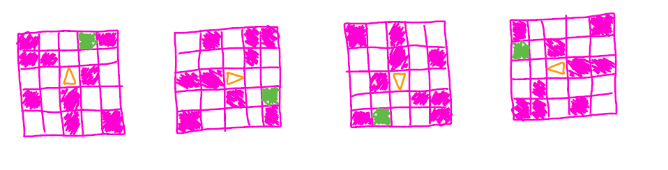
In this case, we have defined the observational frame of reference to be fixed with the world. For consistency, we define the actions to exist in the same frame, yielding the action space \( \mathcal{A}:\) {Move Up, Move Down, Move Left, Move Right} we see that the optimal action to take is different for each observation, meaning the agent has to represent 4 distinct observation/optimal action mappings. Instead, we can choose to set the action and observation spaces in a reference frame attached to the agent (often referred to as a body-fixed frame). In this frame, observations and actions depend on the direction the agent is facing, and one choice for the new action space can be \( \mathcal{A}:\) {Move forward, Rotate clockwise, Rotate counterclockwise, Move backwards}. When using this new reference, we can observe that the four observations and optimal actions above collapse into the leftmost observation and the "Move forward" optimal action. We only need to learn a single optimal action for a single observation, and we have successfully simplified our problem.
Choosing an appropriate frame of reference can be interpreted as a particular case of exploiting the inherent symmetry of a problem when defining the state/observation features. Here, we have used our knowledge of the environment to encode a form of invariance to translations and rotations.
Returns calculation for terminated episodes
What is it?
RL algorithms that use a value network require the returns to be calculated as the target for the value network during training, but we need to handle the time steps when the episode terminated. If the episode terminated, you should not use the returns at the next time step (which is from a new episode) in your calculation because the terminating state has a value of 0 by definition. If the episode terminated because the agent reached a terminal state, you can mask the returns when the episode terminates. For many RL environments, it is also common to set a time-limit to truncate each episode so that it doesn't last too long, or to truncate continuous RL problems to create episodes. For truncated episodes, you can bootstrap using the predicted value of the state instead. This allows the agent to train using the estimate of what the future returns would be at that state if the episode had not been truncated.
When is it useful?
Properly handling the termination of an episode should be implemented with all RL algorithms. However, bootstrapping using the value estimate for the final step on a time-limit truncated episode is an implementation choice. If you choose to truncate because you have a continual problem and want to split into episodes to make learning more practical, you should consider bootstrapping. However, if you use a time-limit to truncate episodes because you want to solve the problem where the task ends at the specified time-limit, then you likely want to avoid bootstrapping and treat the final step as a terminating state.
How to implement it?
You can store the done status at each time step in the same way you store the states and actions for your specific algorithm (e.g. in the replay buffer). Then when you calculate the returns, you can use the done status to mask the returns at the next time step when the episode terminates.
returns[step] = reward[step] + gamma * returns[step+1] * (1-done[step+1])For time-limit truncated episodes, you can can also store masks for truncated episodes. For example, with OpenAI gym, you can use the TimeLimit wrapper:
from gym.wrappers import TimeLimit
env = TimeLimit(env, max_episode_steps)
Using this wrapper, you can determine whether an episode was truncated due to the time limit at each time step and store this information:
truncated_mask = 0.0 if info.get("TimeLimit.truncated", False) else 1.0Then update the return calculation to use the predicted value of the state as the returns when the episode is time-limit truncated, and use the standard returns calculation otherwise.
returns[step] = (reward[step] + gamma * returns[step+1] * (1-done[step+1]))
                * truncated_masks[step+1] + (1-truncated_masks[step+1])
                * pred_value[step]
Reward standardisation
What is it?
Reward standardisation is the process of transforming a given collection of rewards into a standard range. In the case of using function approximators for the value function, a given set of rewards helps form the learning target. Having rewards that vary greatly can create an unstable learning process. Reward standardisation can alleviate this instability by confining the range of values of the learning target.
When is it useful?
Reward standardisation can be helpful if your environment produces rewards with an extreme range of values. For example, rewards can span several orders of magnitude within games in the popular Atari suite. But unfortunately, there is no universal advice for reward standardisation. For example, some environments come with a reward function that caps the possible range of rewards, such as \( [0,1] \). In such cases, reward standardisation is unlikely to make a significant difference in the learning process.
How to implement it?
Rewards can be standardised on a per-episode basis, as shown here:
returns = (returns - returns.mean()) / (returns.std() + eps)In this case, a given episode's collection of rewards are subtracted by their mean and divided by their standard deviation. This forces the rewards to have zero mean and unit variance. Also, rewards can be standardised by using running statistics over the lifetime of an agent, as shown here. Here, the mean and deviation of rewards are updated with every batch throughout training. In contrast to the previous example, this method arrives at values that eventually converge to the "true" summary statistics of the reward function.
Paying close attention to action repeats
What is it?
Many common benchmark environments, such as the PlaNet benchmark suite [1] (based on the DeepMind control suite [2]), use task-specific hyperparameters that affect environment dynamics. One such hyperparameter is action repeat. Action repeat is an important input for RL experiments because it controls the number of times a chosen action repeats at each environment step, which can significantly impact episodic learning. For example, if an environment has an episode length of 1000 steps and an action repeat of four, the agent ultimately chooses 250 actions per episode.
When is it useful?
If you are performing research, it is important to pay close attention to the environment settings of your baselines, especially if you are not running the baselines yourself but instead copying reported figures.
Most RL algorithms perform one update per action selection. Therefore, using a non-standard action repeat value in this paradigm creates an unfair comparison between algorithms. For example, suppose algorithm A uses an action repeat of four while algorithm B uses an action repeat of one. In that case, algorithm B will perform four times the number of weight updates as algorithm A at any given number of environment steps.
How to implement it?
Most environments that use variable action repeat values provide an API through which hyperparameters are set. For example, the dmc2gym API allows users to alter DMControl environments. In the below code block, we first create an instance of the Cartpole, Swingup environment with image-based states. In the PlaNet benchmark suite, this environment has an action repeat of 8 and an episode length of 1000 environment steps, which results in 125 action selections per episode. In dmc2gym, the frame_skip keyword argument sets the action repeat.
import dmc2gym

env = dmc2gym.make(
    domain_name='cartpole',
    task_name='swingup',
    seed=1,
    visualize_reward=False,
    from_pixels=True,
    height=84,
    width=84,
    frame_skip=8,
    camera_id=0
)

done = False
obs = env.reset()

while not done:
    ...
2. Optimisation stability
Orthogonal weight initialisation
What is it?
Orthogonal initialisation (OI) is one of the many options for initialising the learnable parameters of a model. OI has been studied in theory by Hu et al. (2020) [3] in the context of deep linear networks and in practice by Rao et al. (2020) [4] in the context of RL. For a given matrix \( W \in \mathbb{R}^{n \times m} \), OI has three possible initialisation outcomes. If \( n = m \), then \( W^{\top}W = I \). If \( n < m \), then \( W_{i,:} \perp W_{j, :} \; \forall i \neq j \). Finally, if \(n > m\), then \(W_{:, i} \perp W_{:, j} \; \forall i \neq j\).
Most deep learning libraries implement OI based on the work of Saxe et al. (2014) [5], where a semi-orthogonal matrix is formed via QR decomposition. PyTorch’s implementation can be found here, and TensorFlow’s implementation can be found here.
When is it useful?
OI is a sensible initialisation scheme for RL algorithms. Empirically, RL agents initialised with OI lead to higher levels of convergence and more stable training than agents with other initialisation types [4].
How to implement it?
Every deep learning library provides an API through which weights can be initialised. For example, view the below PyTorch code block. Here, we initialise a Linear layer's weight matrix and fill its bias vector with zeros.
from torch import nn

ortho_layer = nn.Linear(16, 32)
nn.init.orthogonal_(ortho_layer.weight)
ortho_layer.bias.data.fill_(0.0)
Similarly, in Tensorflow, OI can be achieved via the below code block.
import tensorflow as tf

oi = tf.keras.initializers.Orthogonal()
ortho_layer = tf.keras.layers.Dense(
    32, kernel_initializer=oi
)
For examples of OI being used in research codebases, see here for OI in the context of Soft Actor Critic and here for OI in the context of A2C and PPO.
Gradient clipping
What is it?
In PyTorch, Gradient clipping rescales the model parameter's gradients so that the norm of a vector containing all of the model gradients gets clamped under some limit. The subtlety here is that while performing gradient clipping results in an upper bound for this norm, it is a rescaling and not a clipping operation that is performed on the individual gradients.
When is it useful?
This technique may be useful if your model is experiencing large or exploding gradients during training. In the context of RL, these large gradients may occur when the training task presents a wide numerical range for its rewards, returns or n-steps returns. Thus, gradient clipping may be a way to obtain some of the benefits of reward or return-standardisation, in cases when normalisation is impractical to implement. More generally, since it acts directly on the individual parameter's gradients, gradient clipping may be helpful to address any cause of exploding gradients, irrespective of the underlying cause, and at little to no computational cost. As such exploding gradients may also be caused by a log probability of an almost 0 probability action that was sampled by the policy, importance sampling weights or the inclusion of a KL divergence term in the loss function.
Lastly, it is important to understand the relationship between gradient clipping and the batch size. A small batch size will create higher variance gradients which are more likely to get clipped. This can be beneficial as this has the additional benefit of reducing the variance of the gradients, but it also means that we introduce a bias in our gradient estimates. In contrast, increasing the batch size is a bias-free method of reducing variance, at the cost of higher computational costs. The choice of batch size and gradient clipping values therefore corresponds to a trade-off between variance, bias and computational complexity.
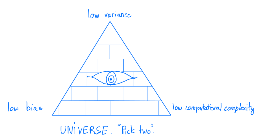
The inescapable trade-off in Machine Learning
How to implement it?
There is a specific PyTorch method for gradient clipping, which makes implementation straightforward:
optimizer.zero_grad()
loss, hidden = model(data, hidden, targets)
loss.backward()

torch.nn.utils.clip_grad_norm_(model.parameters(), args.clip)
optimizer.step()
Target networks
What is it?
Target networks are employed to alleviate the training instability introduced by bootstrapping. They are effectively copies of some reference network (for example the Q-network in DQN [6]) whose weights are either held constant and periodically updated to match their reference network (hard updates) or gradually updated to slowly converge towards the reference network weights (soft updates).
When is it useful?
Because they stabilise the training of value or state-value prediction networks, target networks can be employed in both value and actor-critic methods. In the later, a common misconception is that target networks stabilise the training of both the actor and the critic, since they are usually created for both. However, only the critic's loss employs bootstrapping. As such, they only stabilise the critic's training, as the critic's loss is computed using both the actor's and the critic's outputs.
Target networks are usually only employed in off-policy algorithms. This is because on-policy algorithms are inherently more stable, as they update their value estimates for all visited states, preventing the gradual divergence induced by function approximation and bootstrapping. Nonetheless, target networks may be employed to reduce the variance of the gradient updates. On-policy algorithms are often limited to small batch sizes due to the cost of generating on-policy data, leading to higher variance in the loss computation. A softly-updated target network can be seen as being updated using multiple training batches, since its weight are a moving average of the reference network's. As such, a loss computed using a target network will typically have a lower variance. However, we introduce some bias by doing so, as updates obtained using the target network are not strictly on-policy.
Lastly, it is worth mentioning a specific feature of the TD3 algorithm [7] involving target networks: adding noise to the target actor outputs when computing the value loss results in the smoothing of the action values estimates and prevents the algorithm from prioritising a specific action vector.
How to implement it?
To implement target networks, simply add the soft or hard update functions to your network class and use those to update the weights, instead of the classic (.backwards() -> .step()). Make sure you initialise the reference network and its target as separate objects.
class FCNetwork(nn.Module):

    [...]

    def hard_update(self, source: nn.Module):
        """Updates the network parameters by copying the parameters of
        another network
        :param source (nn.Module): network to copy the parameters from
        """
        for target_param, source_param in zip(self.parameters(),
                                                source.parameters()):
            target_param.data.copy_(source_param.data)

    def soft_update(self, source: nn.Module, tau: float):
        """Updates the network parameters with a soft update
        Moves the parameters towards the parameters of another network
        :param source (nn.Module): network to move the parameters towards
        :param tau (float): stepsize for the soft update
            (tau = 0: no update; tau = 1: copy parameters of source network)
        """
        for target_param, source_param in zip(self.parameters(),
                                                source.parameters()):
            target_param.data.copy_(
                (1 - tau) * target_param.data + tau * source_param.data
            )
3. Multi-Agent Reinforcement Learning (MARL)
Parameter sharing
What is it?
Using one value network (or one policy network) that is shared across all agents can speed up training and is used in the implementation for many MARL papers. With only one network, training is faster because there are fewer parameters to learn and all agents contribute to the updates.
When is it useful?
When implementing MARL algorithms, you should consider whether it is necessary for each agent to have a separate network for your specific problem. If it is not strictly necessary to have separate networks then you can get the speed improvements of using the same network for all agents. However, the downside is that agents can't learn different skills [8] so the suitability of this trick depends on the specific problem.
How to implement it?
You can implement just one value network (or just one policy network) and pass each agent's update through this single network. You may want to also parallelise the forward passes through this network using the tip below. You can also add a one-hot encoding of the agent ID as an additional input to the shared network to allow the network to still learn different functions for each agent.
Common optimiser
What is it?
The optimiser and backpropagation are often implemented separately for each agent to enforce independence between the agents. However, you can implement one optimiser for all parameters and therefore one backpropagation step whilst maintaining independent networks for each agent. This allows PyTorch to optimise the updates internally and it can greatly improve the wall-clock speed.
When is it useful?
This trick can be used to speed up any MARL implementation, even if you have separate networks for each agent.
How to implement it?
When the optimiser is initialised, give it all agent's network parameters to be optimised:
params_list = list(nn_agent1.parameters()) + list(nn_agent2.parameters()) + ...
common_optimiser = torch.optim.Adam(params_list, lr=lr)
During the update step, the losses for each agent can be combined by summing them. Then this combined loss is backpropagated in one step:
total_loss = agent1_loss + agent2_loss + ...
common_optimiser.zero_grad()
total_loss.backward()
common_optimiser.step()
Parallelise forward passes
What is it?
During action selection, you don't have to wait for one agent's forward pass through the neural network to compete before starting the forward pass for the next agent. Instead, you can run the forward passes for all agents in parallel, which can result in in significant speed improvement if you have many agents.
When is it useful?
This trick can be used to speed up any MARL implementation, even if you have separate networks for each agent.
How to implement it?
If all agents share the same network, you can stack the inputs to do a single forward pass of the network. If the agents have separate networks, you can use PyTorch JIT to call each network in parallel and pass their respective inputs. For example, the following code calls a list of agent neural networks in parallel and feeds their respective inputs:
def forward(self, inputs: List[torch.Tensor]):

    futures = [
        torch.jit.fork(model, inputs[i]) for i, model
        in enumerate(self.independent)
    ]

    results = [torch.jit.wait(fut) for fut in futures]
    return results
where self.independent = [nn_agent1, nn_agent2, nn_agent3, ...] is a list of neural networks for each agent, such as value networks.
References
- Danijar Hafner, Timothy Lillicrap, Ian Fischer, Ruben Villegas, David Ha, Honglak Lee, James Davidson (2019). "Learning latent dynamics for planning from pixels". Proceedings of the 36th International Conference on Machine Learning.
- Yuval Tassa, Yotam Doron, Alistair Muldal, Tom Erez, Yazhe Li, Diego de Las Casas, David Budden, Abbas Abdolmaleki, Josh Merel, Andrew Lefrancq, Timothy Lillicrap, Martin Riedmiller (2018). "DeepMind control suite". arXiv preprint: arXiv:1801.00690.
- Wei Hu, Lechao Xiao, Jeffrey Pennington (2020). "Provable benefit of orthogonal initialization in optimizing deep linear networks". International Conference on Learning Representations.
- Nirnai Rao, Elie Aljalbout, Axel Sauer, Sami Haddadin (2020). "How to make deep rl work in practice". NeurIPS Deep RL Workshop.
- Andrew M. Saxe, James L. McClelland, Surya Ganguli (2014). "Exact solutions to the nonlinear dynamics of learning in deep linear neural networks". International Conference on Learning Representations.
- Volodymir Mnih, David Silver, Andrei A. Rusu, Joel Veness, Marc G. Bellemare, Alex Graves, Martin Riedmiller, Andreas K. Fidjeland, Georg Ostrovski, Stig Petersen, Charles Beattie, Amir Sadik, Ioannis Antonoglou, Helen King, Dharshan Kumaran, Daan Wierstra, Shane Legg, Demis Hassabis (2015). "Human-level control through deep reinforcement learning". Nature, (518): 529-533.
- Scott Fujimoto, Herke van Hoof, David Meger (2018). "Addressing function approximation error in actor-critic methods". Proceedings of the 35th International Conference on Machine Learning.
- Filippos Christianos, Georgios Papoudakis, Arrasy Rahman, Stefano V. Albrecht (2021). "Scaling multi-agent reinforcement learning with selective parameter sharing". Proceedings of the 38th International Conference on Machine Learning.